Visualization of Moiré Superlattices by Twist
Here follows a quick view of the commensurate Moiré superlattices composed of twisted homobilayer graphene:
using MoireSuperlattices
using Plots

anim = @animate for i ∈ 2:10
    plot(
        CommensurateBilayerHoneycomb((i, 1)), :real, 30;
        xlim=(-50, 50), ylim=(-30, 30), axis=false, size=(600, 400), vector=false
    )
end
gif(anim; fps=1.5)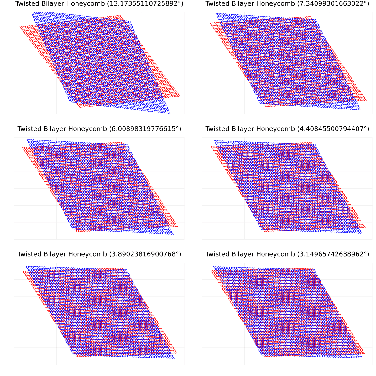
The crystal structure of a commensurate Moiré superlattice composed of twisted homobilayer graphene is characterized by two coprime positive integers (m, r) [Phys. Rev. B 86, 155449 (2012)]. In general, we need to distinguish two cases, i.e., whether gcd(r, 3) is 1 or 3, where gcd denotes the greatest common divisor.
When gcd(r, 3) is 1
For example, m=8, r=1:
plot(CommensurateBilayerHoneycomb((8, 1)), :real; xlim=(-20, 20), ylim=(-10, 20))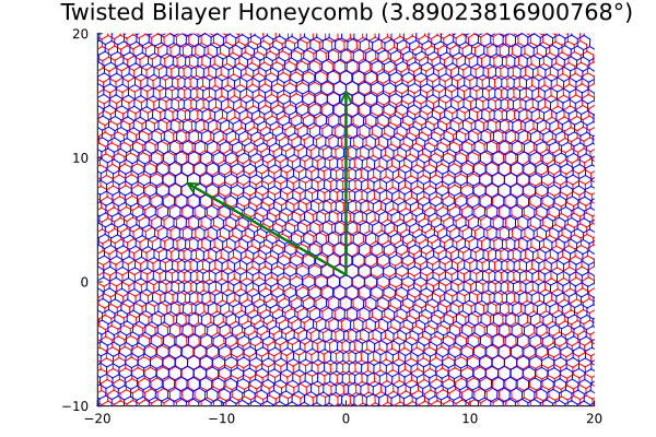
In the reciprocal space, the K points of the top and bottom layers correspond to two inequivalent K points of the Moiré Brillouin zone:
plot(CommensurateBilayerHoneycomb((8, 1)), :reciprocal; xlim=(-5, 5), ylim=(-4, 4))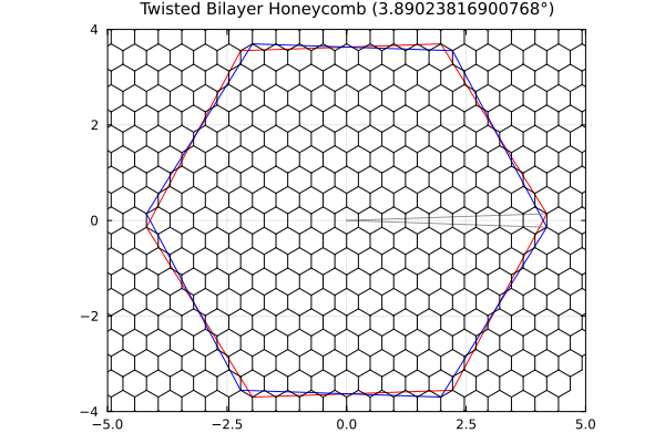
When gcd(r, 3) is 3
For example, m=20, r=3:
plot(CommensurateBilayerHoneycomb((20, 3)), :real; xlim=(-20, 20), ylim=(-10, 20))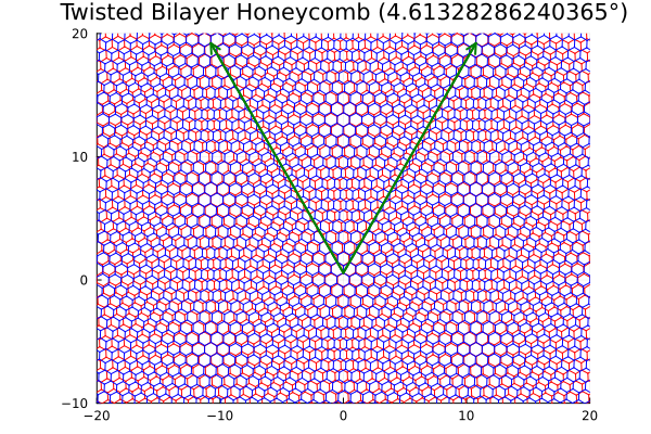
In the reciprocal space, the K points of the top and bottom layers correspond to two equivalent K points of the Moiré Brillouin zone:
plot(CommensurateBilayerHoneycomb((20, 3)), :reciprocal; xlim=(-5, 5), ylim=(-4, 4))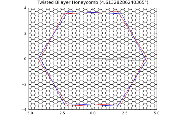
Moiré Reciprocal Lattice with Truncation
In the continuum model, the wavefunction is expanded in a plane-wave basis $\sum_{\mathbf{G}} c_{\mathbf{G}} e^{i(\mathbf{k}+\mathbf{G})\cdot\mathbf{r}}$, where $\mathbf{G}$ runs over the reciprocal lattice vectors of the emergent moiré superlattice. In practice, the sum is truncated to a finite number of shells:
using MoireSuperlattices
using Plots

lattice = MoireTriangularReciprocal(4)
plot(lattice, 1)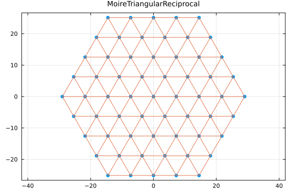
The truncation parameter 4 means all $\mathbf{G}$ vectors with $|\mathbf{G}| \leq 4 \cdot |\mathbf{b}_1|$ are included, where $\mathbf{b}_1$ is the primitive reciprocal lattice vector.